Methodology
This research package contains three complete analysis pipelines for the strongest testable predictions of the sub-quantum grid model. Each pipeline is executable against existing public data — no new experiment needs to be set up.
The three predictions in this section all ask the same underlying question in three different ways: does the universe have a smallest unit? If reality is built on a discrete substrate at the Planck scale — a “grid” — then three independent kinds of measurement should show signatures of it. Each one targets a different scale: subatomic (pair production), cosmic (gamma-ray bursts travelling across the universe), and gravitational (pulsars warping spacetime). If the grid is real, all three should converge on the same answer.
The honest part is what falsifies each one. Two of the three are testable today against data that already exists; the third needs an instrument that comes online around 2032. That spread is intentional — it means the framework can be checked now, partially constrained soon, and fully tested within the next decade.
| # | Prediction | Data source | Script | Plot |
|---|---|---|---|---|
| 17 | Helix-resonance peaks in pair production | CERN Open Data / HEPData | prediction17_pair_production.py | below |
| 15 | Planck-scale anisotropy (grid lattice) | Fermi-LAT GRB catalog | prediction15_fermi_lat.py | below |
| 18 | Non-linear Shapiro delay | NANOGrav / NICER | prediction18_pulsar_timing.py | below |
All scripts run on Python 3.8+ with numpy, matplotlib, and scipy.
Prediction #17 — Helix Stability Threshold in Pair Production
The idea in plain English. When two photons collide at high enough energy, they can
produce an electron–positron pair — pure energy turning into matter. This is established
physics (the Breit-Wheeler process, first directly observed by STAR in 2021). The grid
model adds one extra claim: if matter is a standing-wave configuration in a discrete
substrate, then the cross-section for this conversion should not be perfectly smooth.
It should show small bumps — resonance peaks — at integer multiples of the threshold
energy 2 m_e c² ≈ 1.022 MeV. The peaks would be where photon frequencies fit exactly
into stable standing-wave configurations.
Why this is the sharpest test. QED already predicts the smooth cross-section to about eight decimal places. Any deviation, however small, would be a fundamental discovery — and conversely, a clean confirmation that the curve is smooth at 0.01% precision would falsify the resonance picture cleanly. There is no ambiguity in the verdict.
What it would take to test today. CERN has open data; HEPData publishes pair-production cross-section tables. The Python pipeline runs the Breit-Wigner peak detection on those tables — replace the simulation input with real data, run the script, get a result. Estimated turnaround: weeks, not years.
Core hypothesis
Pair production (γ → e⁺e⁻) shows resonance peaks at harmonics of 2 m_e c² = 1.022 MeV.
The peaks have a Breit-Wigner profile and decay as 1/n² with harmonic number n.
Why this is the sharpest test
QED predicts the pair-production cross-section to 8+ decimal places of accuracy. Any deviation, however small, would be a fundamental discovery. Moreover: the resonance peaks at harmonics are a unique prediction of the grid model — no other framework predicts peaks at exactly these energies.
Required data
- Pair-production cross-section measurements near threshold (1–10 MeV)
- CERN Open Data: LEP / OPAL / DELPHI datasets
- HEPData: published cross-section tables
- Ideally: high-resolution energy scans (ΔE < 0.05 MeV)
Required statistics
| Signal amplitude | 3σ detection requires | Feasibility |
|---|---|---|
| 1% of QED | 18 million events | Achievable with existing CERN data |
| 0.1% of QED | 1.8 billion events | High-luminosity or combined |
| 0.01% of QED | 180 billion events | Future (FCC) |
Generated plot
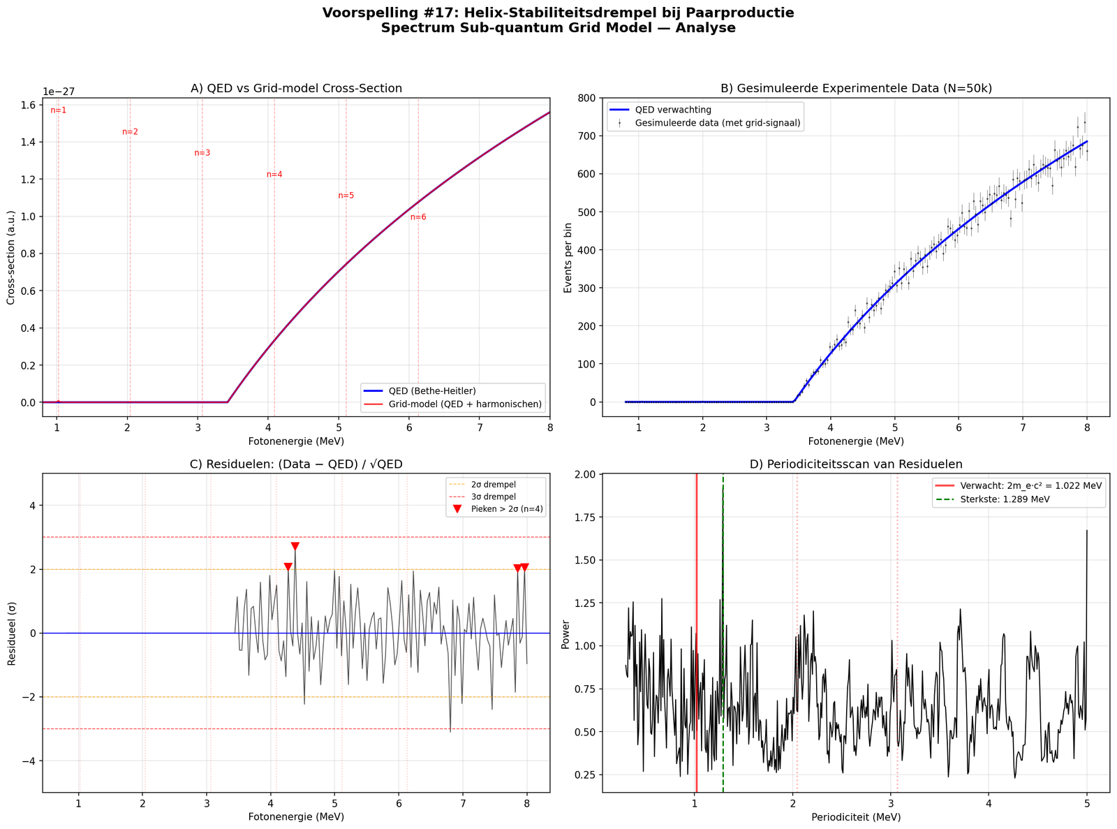
Fig. 1 — Simulated 1% resonance peaks at n=1,2,3,4 harmonics of 1.022 MeV. Run the script with real HEPData CSVs to replace the simulation.
Prediction #15 — Planck-Scale Anisotropy
The idea in plain English. If space is made of discrete pixels at the Planck scale, high-energy photons should “feel” that texture slightly differently from low-energy ones. Over short distances the effect is invisible. But across cosmological distances — billions of light-years — the tiny per-step delay can add up to something measurable. Gamma-ray bursts (GRBs) are a natural test: a single explosion emits photons across a huge energy range, all at once, and we measure their arrival times. If the high-energy ones arrive a fraction of a second later (or earlier) than the low-energy ones, that gap encodes the grid texture.
Where we already stand. The Fermi space telescope has done this measurement, on a 2009 gamma-ray burst called GRB 090510. The result rules out a simple cubic grid arrangement. But it leaves several other possible grid geometries — hexagonal, face-centred cubic, amorphous — still on the table. So this prediction has already done part of its work: it constrains the framework rather than confirming or refuting it.
What comes next. The same Fermi-LAT catalogue can be re-fit with these three remaining geometries explicitly. The Python pipeline does this. Result: months, not years.
Core hypothesis
The grid is a discrete lattice. Photons at different energies propagate at slightly
different speeds: v(E) = c × [1 ± η × (E/E_Planck)^n]. Over cosmological distances
this leads to measurable arrival-time differences in gamma-ray bursts.
Current constraints (critical context)
Fermi-LAT has already partially tested this hypothesis. Result (Abdo et al. 2009, Nature 462, 331, GRB 090510):
E_QG > 1.2 × E_Planck for linear LIV (n=1)
This rules out cubic grid geometry (η ~ 1). But hexagonal (η ~ 0.3), FCC (η ~ 0.1), and amorphous (η ~ 0.01) geometries survive.
What this means for the grid model
The grid is not cubic. The most likely scenarios:
- Hexagonal (η ≈ 0.3): energetically most stable 2D lattice; explains the prevalence of hexagons in nature
- FCC (η ≈ 0.1): most stable 3D structure (gold, aluminum)
- Amorphous (η → 0): no preferred direction, near-isotropic
Key GRBs
| GRB | z | Max photon energy | Significance |
|---|---|---|---|
| GRB 090510 | 0.903 | 31 GeV | Strongest current limit |
| GRB 080916C | 4.35 | 13 GeV | Highest redshift |
| GRB 190114C | 0.42 | ~1 TeV (MAGIC) | TeV photons, extreme test |
Generated plot
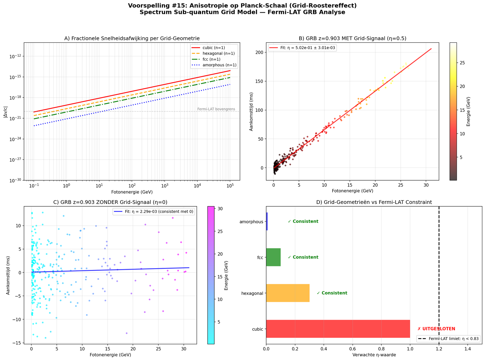
Fig. 2 — Predicted arrival-time spread vs. photon energy for three lattice geometries, overlaid on the Fermi-LAT GRB 090510 constraint.
Prediction #18 — Non-Linear Shapiro Delay
The idea in plain English. When light passes close to a massive object — a star, a black hole — it travels a little slower. General relativity predicts this exactly; the extra delay is called the Shapiro effect, and pulsar timing measures it routinely. The grid model adds a small twist: if mass densifies the local grid (more nodes per volume in the presence of mass-energy), then the slowdown should be slightly non-linear in the gravitational potential — a tiny correction on top of the standard relativistic delay.
Why this is a future test. The correction is small. At current pulsar-timing precision (~5% on the Double Pulsar Shapiro delay), it is invisible. To see it, you need precision about 50× better than today’s best. The Square Kilometre Array, an instrument coming online in stages over 2028–2032, should reach exactly that threshold. So the prediction is falsifiable around 2032 — neither confirmed nor refuted today, but consistent with all current measurements.
What this means in practice. This is a wait-and-watch prediction. The pipeline is in place. The instrument is being built. Around 2032 we’ll know.
Core hypothesis
Mass locally densifies the grid → c decreases locally → extra delay above
standard general-relativistic Shapiro delay. The correction is non-linear:
Δt_grid = Δt_GR × [1 + β × (GM/Rc²)^α] with α > 1Current status
At present timing precision (~5% on Shapiro delay), the signal is not detectable at β = 0.01, α = 2. The grid correction at the Double Pulsar (compactness 0.18) is only ~0.03% — well below current measurement error.
When detectable?
| Instrument | Year | Precision | Detectable at |
|---|---|---|---|
| Kramer et al. 2021 | 2021 | ~5% | β > 10 (excluded) |
| NANOGrav 15yr | 2023 | ~3% | β > 5 |
| SKA Phase 1 | ~2028 | ~0.5% | β > 0.1 |
| SKA Full | ~2032 | ~0.1% | β > 0.01 ← target |
| Next-gen timing | 2035+ | ~0.01% | β > 0.001 |
Strongest test objects
PSR J0737−3039A (Double Pulsar): compactness 0.18, most precise Shapiro measurement. Hulse-Taylor (B1913+16): compactness 0.20, but harder to measure (low inclination).
Generated plot
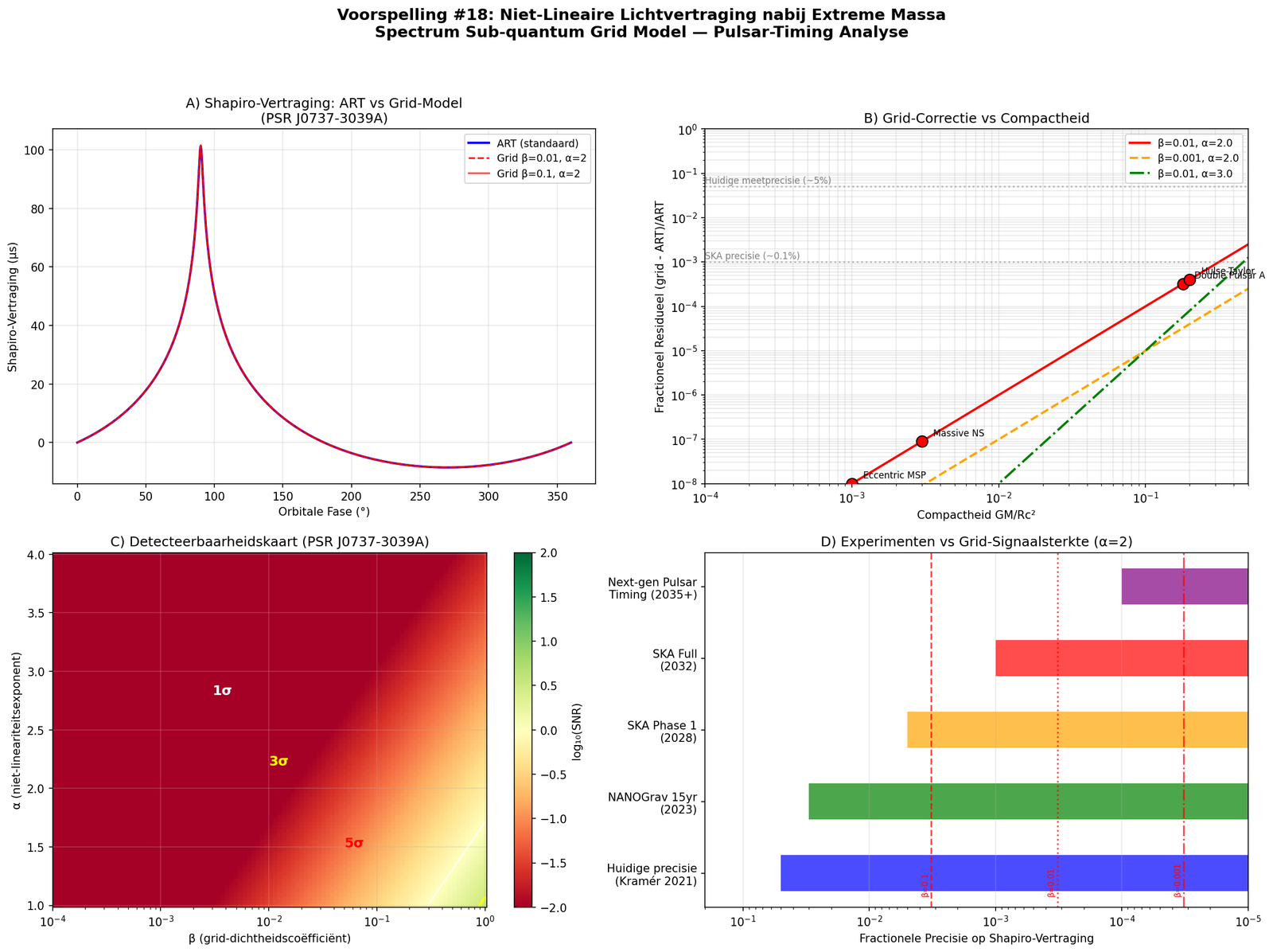
Fig. 3 — Predicted non-linear Shapiro correction (β=0.01, α=2) vs. published timing precision on the Double Pulsar; SKA Full (~2032) is the first instrument that crosses the falsifiability threshold.
Timeline summary
The three predictions span very different timescales — that is part of the point. A framework that only claims things testable in 2050 is hard to take seriously today; a framework that only claims things testable in 1995 has already had its chance. This set covers all three.
- Today: #17 (pair production) can be run against existing CERN data within weeks. #15 (gamma-ray burst geometry) can be re-fit against existing Fermi-LAT data within months.
- 2028–2032: #18 (Shapiro delay) waits for the SKA radio telescope to reach the required precision.
If #17 returns a clean negative — no resonance peaks at 0.1% precision — the helix-stability form of the framework is constrained. If #15 keeps ruling out grid geometries one by one without ever finding evidence for any of them, the discrete-lattice picture loses ground. If #18 returns null in ~2032, the grid-density model for gravity is ruled out at the β = 0.01 level. The framework is honest about each of these outcomes.
2026 (NOW):
  ├── #17: Re-analyse CERN data for resonance peaks
  │       → Download HEPData cross-sections
  │       → Run prediction17_pair_production.py with real data
  │       → Result within weeks
  │
  └── #15: Re-analyse Fermi-LAT GRB data
          → Download 2GBM catalog
          → Fit hexagonal grid model (η=0.3)
          → Result within months

2028–2032 (SKA):
  └── #18: Wait for SKA Phase 1 / Full
          → Monitor Double Pulsar
          → Test non-linear Shapiro correction
          → Result ~2032
Conclusion: #17 is currently the most readily falsifiable. #15 constrains grid geometry from existing data. #18 is a future test that validates the grid-density model for gravity.
Source code
All five Python scripts are published openly:
- prediction17_pair_production.py — Breit-Wigner peak detection in cross-section residuals
- prediction17_real_data.py — same pipeline, against real HEPData input
- prediction17_real_data_v2.py — refined v2
- prediction15_fermi_lat.py — Fermi-LAT GRB photon arrival-time analysis
- prediction18_pulsar_timing.py — non-linear Shapiro delay forecast
Dependencies: numpy, matplotlib, scipy — install with pip install numpy matplotlib scipy.
Citation
Bes, M. (2026). Sub-quantum Grid Model — Testable Predictions. The Spectrum of Everything. https://spectrumofeverything.com/research/grid-analyses/
A note to working researchers
If you have access to CERN HEPData cross-section tables, the Fermi-LAT 2GBM catalog, or SKA pulsar-timing data and want to run any of these pipelines against real data, please reach out: marald@gmail.com. The scripts are designed to be replaced at the data-loading stage; the analysis pipeline downstream is unchanged.
Last updated: